Separating Hyperplanes

No evidence of declining volatility for Bitcoins

Matthew Martin 1/22/2014 10:43:00 PM

Chart showing Eli Duorado's OLS regression, which suggests that the volatility is falling over time.

Eli Dourado has a post up arguing that the volatility of the returns on Bitcoin are falling. As evidence, Dourado calculated an OLS regression of Bitcoin volatility over time, and showed that the coefficient was negative and statistically significant. [I want to interject with some public shaming, because Dourado did this using Stata instead of on an open-source platform like R or Python--on a post about Bitcoins no less! Science wants to be free and open!] For clarity, by "volatility" Dourado means specifically the 30-day rolling standard deviation of daily returns (and by "returns" we mean the difference in the natural logs of the daily close prices of a Bitcoin in USD). There are lots of other ways to measure volatility, and it isn't totally clear this is the one we should care about. At any rate, you can see Dourado's regression in the chart above.

Now here's Robert Sams, in rebuttal:

"But the claim that “there is a clear trend of falling volatility over time” isn’t defensible at all."

Sams replicated Dourado's results, and then did his own analysis to suggest that Dourado's regression wasn't valid. In particular, Sams ran essentially the same regression, but on a rolling 2-year window to show how the coefficient estimate is evolving over time as new data comes in:

Sams's results, showing that the OLS coefficient is not a consistent estimator.

Sams adds:

"I don’t like using trend lines in analysing financial timeseries."

No, I suppose I don't like that either.

Listen, we have a term for time series whose time-trends shift over time--it's "non-stationary." How did two economists do regressions on a time series, and yet no one has 1)tested for stationarity or 2)done any time-series econometrics? We have tools for these kinds of questions!

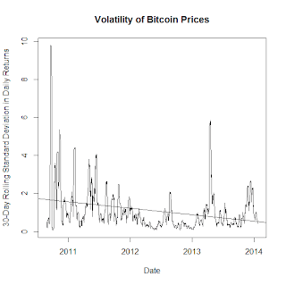
Ok, now that I'm done snarking, I will say that Sams is exactly correct, if a little imprecise. Dourado's error is in assuming that the series he was regressing was stationary when such an assumption cannot be supported. Like Sams, I have also replicated Dourado's results:

And here's my code in R (you need to have the TTR library installed):

library(TTR)
bit = read.table("http://blockchain.info/charts/market-price?showDataPoints=false&timespan=all&show_header=true&daysAverageString=1&scale=0&format=csv&address=",header=FALSE, col.names=c("Date","Close"), fill=TRUE,sep=",")
bit$Date<- as.Date(bit$Date,"%d/%m/%Y %H:%M:%S")
subbit = bit[which(bit$Close>0),]
ohlc <- subbit[,"Close"]
subbit$vClose <- volatility(subbit$Close, calc="close", N=365)
sub2bit = subbit[which(subbit$vClose>=0),]
ols=lm(sub2bit$vClose~sub2bit$Date)
plot(sub2bit$Date, sub2bit$vClose, xlab="Date", ylab="30-Day Rolling Standard Deviation in Daily Returns", type="n", main="Volatility of Bitcoin Prices")
lines(sub2bit$Date, sub2bit$vClose, type="l")
lines(sub2bit$Date, sub2bit$predict, type="l")
abline(ols)
summary(ols)

Notice how many fewer lines that took than Stata...

Now, the problem with Dourado's model is that the data aren't stationary, so his coefficient is not a consistent estimator of the true time trend. It turns out that there's a clever little function on R to test this:

library(forecast)
ndiffs(sub2bit$vClose, alpha=0.05, test=c("kpss", "adf", "pp"))

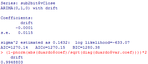
That tells us we need to difference the volatility series before we can say anything about the trends. If your curious, the data failed the Kwiatkowski–Phillips–Schmidt–Shin test, though not the Augmented Dickey-Fuller test for a unit root.

Ok, let's look at this from a different angle. A more precise description of Dourado's hypothesis is that the time-trend in question has a below-zero drift term in the data-generating process. Well, here's that:

In principle, the drift coefficient here should be identical to Dourado's coefficient. Yet, because this series is stationary and Dourado's isn't, we can now see that the coefficient is not statistically significant at all. I've calculated a p-value though it's not part of R's standard output--from the looks of it, the probability is quite low that the time trend *isn't* actually zero.

Of course, since this is a likelihood estimation, model selection should really be based on one or another information criterion, not on individual p-values. So just for kicks, here's the (stationary) time-series model that minimizes the Bayesian-schwarz information criterion:

What actual time-series econometrics looks like.

Oh, look at that--no drift term!

The bottom line here is that Dourado aint got it. I cannot tell you which way Bitcoin volatility is going, but I can tell you that Dourado can't either.

Full R code below:

library(TTR)
bit = read.table("http://blockchain.info/charts/market-price?showDataPoints=false&timespan=all&show_header=true&daysAverageString=1&scale=0&format=csv&address=",header=FALSE, col.names=c("Date","Close"), fill=TRUE,sep=",")
bit$Date<- as.Date(bit$Date,"%d/%m/%Y %H:%M:%S")
subbit = bit[which(bit$Close>0),]
ohlc <- subbit[,"Close"]
subbit$vClose <- volatility(subbit$Close, calc="close", N=365)
sub2bit = subbit[which(subbit$vClose>=0),]
ols=lm(sub2bit$vClose~sub2bit$Date)
plot(sub2bit$Date, sub2bit$vClose, xlab="Date", ylab="30-Day Rolling Standard Deviation in Daily Returns", type="n", main="Volatility of Bitcoin Prices")
lines(sub2bit$Date, sub2bit$vClose, type="l")
lines(sub2bit$Date, sub2bit$predict, type="l")
abline(ols)
summary(ols)
library(forecast)
ndiffs(sub2bit$vClose, alpha=0.05, test=c("kpss", "adf", "pp"))
vCloseArima=auto.arima(sub2bit$vClose, ic="bic")
vCloseArima
(1-pnorm(abs(vCloseArima$coef)/sqrt(diag(vCloseArima$var.coef))))*2
dourado=Arima(sub2bit$vClose,order=c(0,1,0), include.drift=TRUE)
dourado
(1-pnorm(abs(dourado$coef)/sqrt(diag(dourado$var.coef))))*2